Incremental Database Computations

Introduction

In previous blog posts we have:

• informally introduced incremental computation,

• introduced Z-sets as a representation for database tables and changes to database tables.

In this blog post we explain how an incremental query engine like Feldera actually operates as seen by a user. We start by motivating the need for incremental computation in databases. Future blog posts will describe the internal operations in detail.

Periodic queries and views

Many data analysis systems need to periodically execute the same computation on changing datasets. Several examples are:

• Generating company financial reports every quarter that include the data for the latest reporting period.

• Generating weekly inventory reports for stores to decide how to resupply them.

• Generating a new web search index that includes the latest crawled pages.

• Generating a dashboard with interactive visualization for monitoring the power consumption in the electric grid.

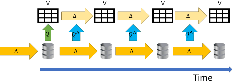
We have ordered these examples in order of increasing frequencies. In all these cases we have a database that stores the data, which keeps changing, and a set of queries that are evaluated periodically to produce results reflecting the latest changes. The following diagram illustrates this process:

The horizontal axis shows the evolution of time. The silver cylinder is a database that keeps changing. Let's assume that the database is very large (1 billion rows), while each of the changes only modifies a small part of the database (100 rows, across one or multiple tables); we use the Greek letter "delta" (Δ) to indicate a change. ΔDB is a change to the database. The diagram shows how a query $Q$ is executed repeatedly and produces some result V.

Incremental view maintenance (IVM)

One mechanism that databases have for describing such repeated queries are database views. Views are nice. They look like database tables, since they can be used as inputs to queries. Their contents changes automatically when tables in the database are modified.

An important question in databases is: how to efficiently recompute the contents of views when the underlying tables change. Database people call this problem Incremental View Maintenance.

The basic idea behind incremental view maintenance is shown in the following diagram:

Since the database changes are very small, instead of computing the contents of the view V every time by re-running the query, maybe we can instead compute only what changes in the view itself, shown as yellow arrows at the top, labeled ΔV. An increment is a change, what we denote by Δ -- that's where the I in IVM comes from. If we can compute ΔV looking only at ΔDB, then we can potentially do it much faster. The emphasis is on much: since DB has 1 billion rows, and ΔDB only 100, this means 10 million times faster! The potential savings are humongous. The goal of the people building IVM systems is to convert the query $Q$ into a new kind of query $Q^\Delta$ which computes ΔV from ΔDB.

The core technology of Feldera is in fact the algorithm which produces $Q^\Delta$ from a query $Q$. That technology is described in detail in our award-winning paper published at the Very Large Databases conference in 2023.

Why IVM is difficult

The IVM problem has been studied for a very long time, and there are many interesting optimizations proposed that work for specific kinds of queries. What our paper does is to propose a universal solution, that works well pretty much for any query you can write.

Superficially this looks like another query optimization problem. Optimizing the execution of queries is the bread-and-butter of databases. So why don't databases do a good job at IVM? The answer is that the IVM queries $Q^\Delta$ differ in a very subtle way from the standard $Q$ queries: while a query $Q$ computes on tables, a query $Q^\Delta$ computes on changes. Unlike tables, changes can be negative: a change can both insert and remove rows from a table. While $Q$ can be described in terms of operations on tables, $Q^\Delta$ can only be described in terms of operations on Z-sets. Notice that changes that update only parts of a row can be described in terms of changes that delete the old row and insert a new version of it.

This is why we spent several blog posts describing how various database computations can be implemented on Z-sets.

As we said, views are nice, because they look like tables. However, what happens if a view itself is very large (let's say 1 million rows)? Even the process of extracting information out of the view is costly (unless the view has indexes). In many applications it may be beneficial if the database system directly provides its consumers the changes to the view ΔV instead of giving access to the view through queries. Often the changes to a view can also be significantly smaller than the view itself. But again, changes can be negative, and databases are very clumsy at representing negative changes. A fair amount of complexity of Change-Data Capture systems deals with representing negative changes.

Feldera only provides outputs consisting of view changes.

Example

Let's see a concrete example in action.

Example using a traditional database

First let's use a traditional database. You can run this example in Postgres, or using a database playground on the internet.

Let's assume we have a CUSTOMER table with two columns: person and zip, which was created by a SQL statement such as:

CREATE TABLE CUSTOMER(
    name VARCHAR NOT NULL,
    zip INT NOT NULL
);

Let's consider a simple query to find out how customers are distributed among zips:

CREATE VIEW DENSITY AS
SELECT zip, COUNT(name)
FROM CUSTOMER
GROUP BY zip;

Right after creating the CUSTOMER table, it is empty. If we inspect the view DENSITY we observe that it is also empty:

SELECT * FROM DENSITY

(0 rows)

Let's insert a few records into the table:

INSERT INTO CUSTOMER VALUES
  ('Sue', 3000),
  ('Mike', 1000),
  ('Pam', 2000),
  ('Bob', 1000);
SELECT * FROM DENSITY;

  zip   count
--------------
 1000       2
 2000       1
 3000       1
(3 rows)

When we inspect the view we observe that it already contains some data.

Now let's assume that Bob moves from zip 1000 to zip 2000. This can be described as a series of updates to the table:

DELETE FROM CUSTOMER WHERE name = 'Bob';
INSERT INTO CUSTOMER VALUES ('Bob', 2000);
SELECT * FROM DENSITY;

 zip    count
--------------
 1000       1
 2000       2
 3000       1
(3 rows)

Notice that the view has changed.

Incremental execution example

We will now execute the same sequence of operations, but in an incremental way. You can try this example using the instructions provided in the tutorial. (Soon we will also offer an on-line playground where you can test such programs without needing to install them on your machine.)

Let's first add an empty change to the table CUSTOMER:

CUSTOMER change:
  empty
DENSITY change:
  empty

As we expected, if we don't change the CUSTOMER table, there is no change in the DENSITY view.

Now let us make a change to CUSTOMER by inserting four rows. This change is a Z-set, where we indicate the weight of each row as a number at the end of the line. +1 shows that rows are inserted:

CUSTOMER change:
  ('Mike', 1000) +1
  ('Pam',  2000) +1
  ('Bob',  1000) +1
  ('Sue',  3000) +1
DENSITY change:
  (1000, 1)      +1
  (2000, 2)      +1
  (3000, 1)      +1

The output produced is a Z-set, with three rows. Each row has a weight of +1, since it has been added to the result. If you were expecting the following result you may be disappointed:

DENSITY change:
  1000 +1
  2000 +2
  3000 +1

The DENSITY view has two columns, one for the zip and one for the count. count is a column, and not a weight. The weight "metadata column" is separate.

Let's apply one more change, moving Bob as before from zip 1000 to zip 2000. This change can be expressed as an insertion of the old record with weight -1 (which is equivalent with a deletion) and an insertion of the new record with weight +1.

CUSTOMER change:
   ('Bob', 1000)  -1
   ('Bob', 2000)  +1
DENSITY change:
   (1000, 1)      -1
   (2000, 2)      -1
   (2000, 1)      +1
   (1000, 2)      +1

Notice how the output change contains two changes for zips 1000 and 2000. To make the correction, the previous value of the row is removed (using a weight of -1) and a new version of the row is inserted (with weight +1).

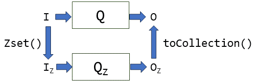
The following diagram shows the time evolution of our example database (which only contains one table, CUSTOMER) and of the DENSITY view. In blue we show tables, and in orange we show Z-sets, which are the changes applied to the tables. Remember that a table can be also expressed as a Z-set. An incremental query engine that computes on Z-sets can thus perform both the computations on the top side and on the bottom side. (This example would also use indexed Z-sets to compute the GROUP BY part of the query.)

The database in this example is small, and the changes we make are about the same size as the database itself. However, as the database size grows, the blue arrows can still be implemented to compute their results by doing work proportional to the number of changed records.

In future blog posts we will discuss how the blue arrows $Q^\Delta$ can be implemented.

Conclusions

An incremental query engine can offer tremendous performance and cost benefits compared to a traditional database. The larger the data, the more frequent the changes, and the more complex the queries, the larger the benefits that can be expected. These benefits come from a reduced computational complexity: the savings expected are roughly proportional to the ratio between the database size and the change size. These savings can be obtained by computing directly on changes, by using Z-sets as a representation.