
Introduction: query engines
Feldera is essentially a SQL query engine. There are countless query engines; each database includes a query engine, and there are even more query engines that are not part of a traditional database, e.g. Apache Spark. The query engine is the component of the database that is given a query written in the SQL programming language and which computes the result of that query based on the current content of the database.
What differentiates Feldera from most existing query engines is the focus on incremental view maintenance. The main use case for Feldera is when users have a continuously-changing database but a slowly changing set of queries. The second time a query is evaluated, Feldera takes advantage of information acquired during the prior execution to compute the result faster than a traditional database would do. Feldera does that by only computing what has changed from the previous computation.
The SQL language is composed from a set of primitive operations that all compute on data collections (also called relations); these operations are named SELECT, WHERE, JOIN, GROUP BY, etc. A SQL query is composed of a combination of these operations.
Consider the following query:
SELECT a+b FROM T
WHERE a > 0
This query is composed of three operators, executed in the following order:
FROM, which reads data from tableTWHERE, which eliminates all rows of tableTwhereais not positiveSELECT, which adds up the data in columnsaandbof each remaining row
Standard query engines implement query evaluation by compiling SQL programs into a dataflow graph representation, optimizing this representation, and then executing this representation by feeding the data in the database as inputs.
What is a dataflow graph? It is a representation of a program composed of two kinds of objects: nodes and edges. Nodes represent computations, and edges show how data flows between nodes. Dataflow graphs can be represented visually as networks of boxes and arrows: the boxes are the computations, which the arrows show how data produced by a node is consumed by other nodes. For SQL programs you can think of the nodes as roughly representing the SQL primitive operations, while each edge represents a collection: the result produced by the node when it receives inputs.
The dataflow graph for the previous query is the following:

Feldera's query engine works in a very similar way. The Feldera SQL compiler has two stages: in a first stage it uses the Apache Calcite infrastructure to compile the query into a query plan, which is optimized using the Calcite optimizer. Afterwards the plan is converted to an incremental plan, where each operator is substituted with an operator that does not compute on collections, but rather on changes, which are described by Z-sets.
Unlike database queries, Feldera queries are supposed to run continuously, each receiving many input changes and producing many output changes. So Feldera queries are compiled into a pipeline, which then runs for a long time, receiving inputs and producing outputs.
Performance profiling
As you can see, there is a long way between the program you write (in SQL) and the program that will be executed to process the data (the pipeline). What can you do if your program is too slow, or requires too many resources (runs out of memory or disk space)? How can you understand where the problems are and how can you perhaps rewrite the program to make it more efficient?
Until recently there was no easy way for Feldera end users to answer this question. Even experienced members of the Feldera team had to spend an inordinate amount of time to understand and troubleshoot the behavior of programs. No longer! Enter the Feldera profiling visualization tool.
Profiling in programming is the technique of measuring and understanding the
behavior of computer programs.
Instrumentation code
We added lots of instrumentation code which collects measurements about the behavior of each operator in a pipeline. These measurements are aggregated into measurement statistics. For example, the pipeline will measure how much time an operator spends to process each change. During the lifetime of a pipeline each operator may be invoked millions of times, so the information is summarized, for example, as the "total time" spent executing this operator.
There are many interesting measurements that may be collected: how much data is received by the operator, how much data is produced by the operator (note that an operator like WHERE produces less data than it receives), how much data was written to disk, how much memory was allocated by an operator, when searching for a value what is the success rate (for JOIN operations), etc.
Multi-core execution
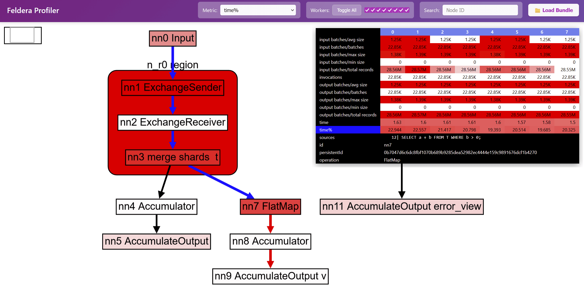
Feldera pipelines are designed to take advantage of multiple CPU cores (and soon will be also be able to take advantage of multiple computers). When you start a pipeline you specify a number of cores, and each operator of the dataflow graph is instantiated once for every core. Sometimes, data needs to be moved between cores, and then a special operator called exchange is used. When you allocate 2 cores, the previous pipeline may actually look like the following picture:

The exchange operator is the dotted box which has the cross-arrows showing data movement between cores.
During execution each of the cores will collect separate profiling measurements.
A large SQL program can be composed of a thousands of operators, each of which can be executed on tens of cores, and each of which can collect hundreds of measurements. How can we make sense of all this data?
Visualizing profiles
We built a tool to graphically display the performance data produced by a running pipeline and to allow users to interactively browse this data. We describe here only the core capabilities of this tool, because it is still under very active development, and the actual user interface and features are still changing.
The profile visualization tool lets you display the dataflow graph of the program. The following screenshot shows the dataflow graph for our little example program:

You will notice that there are two subgraphs: the one on the left has been created by the compiler, and shows how the content of the system built-in error_view is produced (for this program the content is always an empty constant - there can be no errors). The graph on the right is from the SQL program itself.
This dataflow graph actually has two outputs: one for the view v on the right, and one for the input table t itself. Each table has automatically an attached view which allows the user to monitor the table's content.
A drop-down box allows you to select any of the collected metrics:

The nodes in the graph are colored according to the selected metric: nodes are white when the metric is low, and nodes are red when the metric is high, with various shades of pink to show values in between. For the previous program the currently selected metric is time%; this means that the red nodes are the places where most of the execution time is spent.
Various pieces of information can be overlaid on top of the dataflow graph. For example, hovering or clicking on a node in the graph will display all the metrics collected during the program's execution for that node. These metrics are displayed as a table, with one column for each core:

Because this table has 8 data columns, it follows that this program was executed on a machine with 8 CPU cores.
In addition, information such as the original approximate SQL source code position for the node is displayed if it is available:

When hovering with the mouse over a node, or clicking over a node, the reachable nodes through the graph are displayed by coloring incoming (blue) and outgoing (red) edges:

Some dataflow graph operators are actually little graphs themselves; these are displayed as boxes with rounded corners. The following image shows a region named n_r0 region which expands to three operators, implementing the Feldera version of the exchange operator described above. (This operator has 3 stages: send, receive, and merge). Double-clicking on such operators will expand them further. Double-clicking on an expansion will contract it again.

The profiling data can be collected directly from a running job or by saving a support bundle. The profiling data is saved in a json file, and it can be sent for troubleshooting remotely, without requiring direct access to the cluster where the pipelines are running.
In future articles we will describe various use cases for using the profiler to troubleshoot performance problems and optimize programs.