Part 1: Writing and testing your first SQL program

In this section of the tutorial we will:

• Write and test our first SQL program using Feldera
• Introduce continuous analytics -- one of the key concepts behind Feldera

The use case

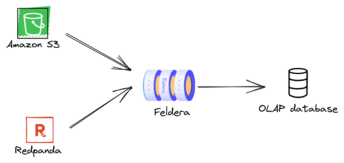
We will use Feldera to implement a real-time analytics pipeline for a supply chain management system. The pipeline ingests data about suppliers, customers, and orders, and maintains an up-to-date summary of this data in an OLAP database. The data can arrive from a variety of sources, such as databases and event streams. In this tutorial we will ingest data from Amazon S3 and Redpanda, a Kafka-compatible message queue.

Step 0. Launch Feldera

Make sure that you have Feldera up and running by following the Getting Started guide. Open the Feldera Web Console on localhost:8080.

For the impatient

If you started Feldera using the demo profile as described in the Getting Started guide, it has created a couple of SQL programs and pipelines. One of these programs, called "Feldera Basics Tutorial" and the associated pipeline "Feldera Basics Tutorial Pipeline" are identical to the ones we will manually create in this three-part tutorial.

We recommend that you follow the tutorial and build your own Feldera pipeline, but if you'd like to accelerate the journey, feel free to skim the tutorial and explore the resulting pipeline without going through all the steps.

Step 1. Declare input tables

We start with modeling input data as SQL tables. In the Feldera Web Console, navigate to the SQL Programs section and click on ADD SQL PROGRAM. Give the program a name, e.g., "Supply Chain Analytics" and paste the following code in the SQL editor:

create table VENDOR (
    id bigint not null primary key,
    name varchar,
    address varchar
);

create table PART (
    id bigint not null primary key,
    name varchar
);

create table PRICE (
    part bigint not null,
    vendor bigint not null,
    price decimal
);

This looks familiar, just plain old SQL CREATE TABLE statements. Indeed, SQL's data modeling language works for streaming data just as well as for tables stored on the disk. No need to learn a new language: if you know SQL, you already know streaming SQL!

It is worth pointing out that these declarations do not say anything about the sources of data. Records for the VENDOR, PART, and PRICE tables could arrive from a Kafka stream, a database, or an HTTP request. Below we will see how our SQL program can be instantiated with any of these data sources, or even multiple data sources connected to the same table.

Step 2. Write queries

We would like to compute the lowest price for each part across all vendors. Add the following statements to your SQL program:

-- Lowest available price for each part across all vendors.
create view LOW_PRICE (
    part,
    price
) as
    select part, MIN(price) as price from PRICE group by part;

-- Lowest available price for each part along with part and vendor details.
create view PREFERRED_VENDOR (
    part_id,
    part_name,
    vendor_id,
    vendor_name,
    price
) as
    select
        PART.id as part_id,
        PART.name as part_name,
        VENDOR.id as vendor_id,
        VENDOR.name as vendor_name,
        PRICE.price
    from
        PRICE,
        PART,
        VENDOR,
        LOW_PRICE
    where
        PRICE.price = LOW_PRICE.price AND
        PRICE.part = LOW_PRICE.part AND
        PART.id = PRICE.part AND
        VENDOR.id = PRICE.vendor;

In Feldera we write queries as SQL views. Views can be defined in terms of tables and other views, making it possible to express deeply nested queries. In this example, the PREFERRED_VENDOR view is expressed in terms of the LOW_PRICE view.

Step 3. Run the program

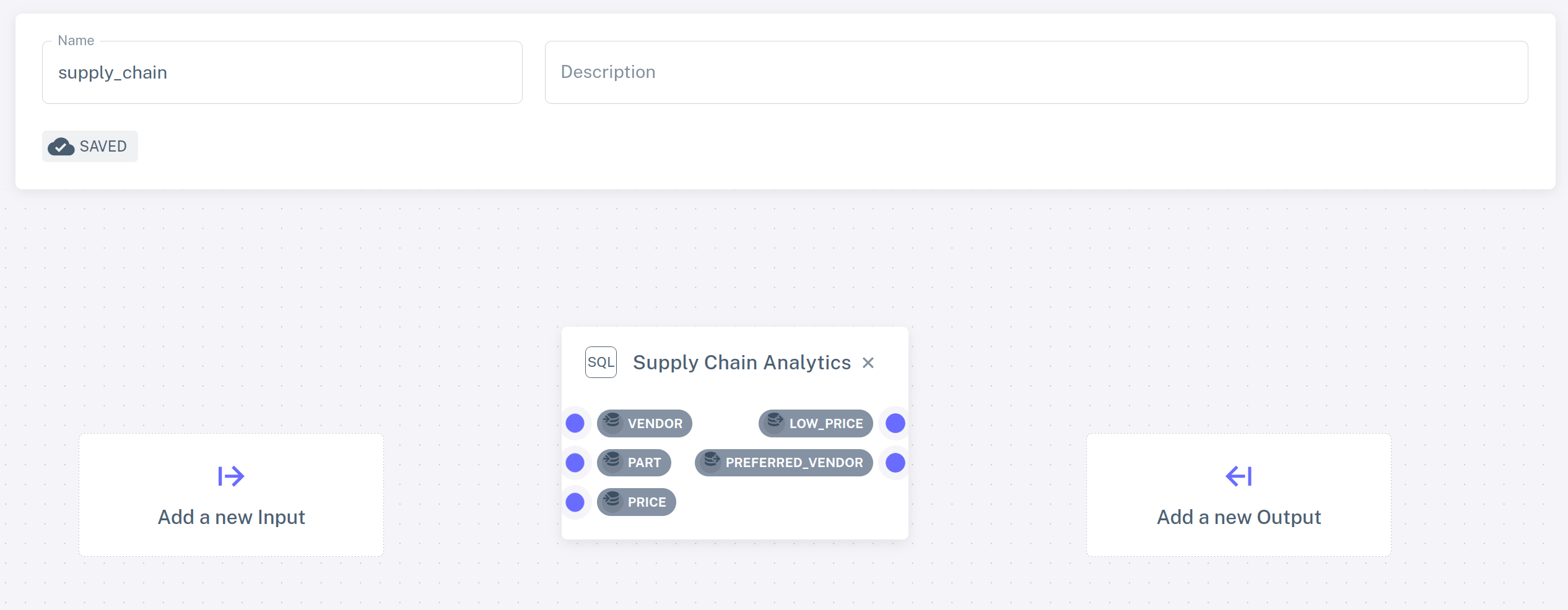
In order to run our SQL program, we must instantiate it as part of a pipeline. Navigate to the Pipelines section and click ADD PIPELINE. Give the new pipeline the name supply_chain and select "Supply Chain Analytics" from the list of SQL programs.

The selected program is visualized as a rectangle with a blue dot for each table and view declared in the program. These can be used to connect data sources and sinks. For the time being, we will run our pipeline without any sources or sinks. We will build more exciting pipelines in the next part of the tutorial.

Go back to the pipelines view (click on Pipelines in the navigation bar on the left). Your newly created pipeline should appear in the list. Click the play icon next to the pipeline.

The pipeline is now running and is ready to process inputs; however since we have not connected any data sources to it, no data has been received yet. Let us add some manually.

Step 4. Populate tables manually

Expand the runtime state of the pipeline by clicking the chevron icon on the left. You should see the list of tables and views defined in your program. Click on the icon next to the PART table. This will open a view with BROWSE PART and INSERT NEW ROWS tabs. The BROWSE PART tab should be empty because no data has been inserted yet. Click INSERT NEW ROWS, where you can insert new rows to the table using a configurable random data generator (feel free to play around with it!) or by entering the data manually. For example, you might add the following rows:

ID	NAME
1	Flux Capacitor
2	Warp Core
3	Kyber Crystal

Click INSERT ROWS to push the new rows to the table. Switch to the BROWSE PART tab to see the contents of the table, which should contain the newly inserted rows.

Follow the same process to populate VENDOR:

ID	NAME	ADDRESS
1	Gravitech Dynamics	222 Graviton Lane
2	HyperDrive Innovations	456 Warp Way
3	DarkMatter Devices	333 Singularity Street

and PRICE:

PART	VENDOR	PRICE
1	2	10000
2	1	15000
3	3	9000

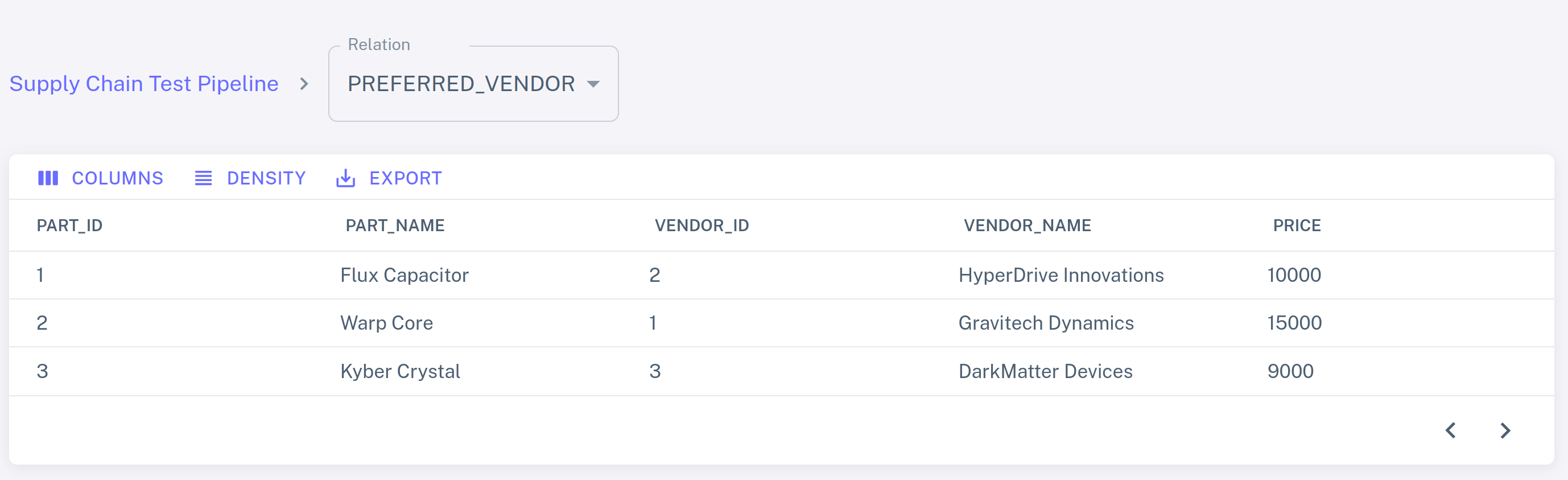
Select the PREFERRED_VENDOR view from the dropdown list to see the output of the query:

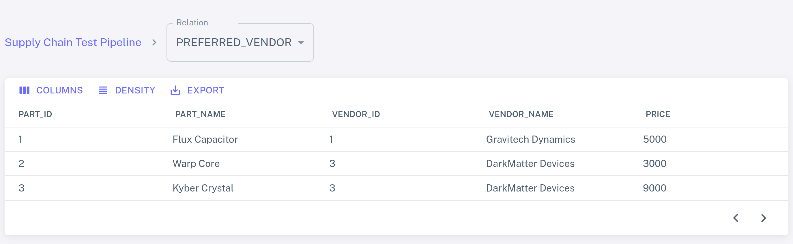
Step 5. Make changes

Let us see what happens if we add more input rows to the PRICE table:

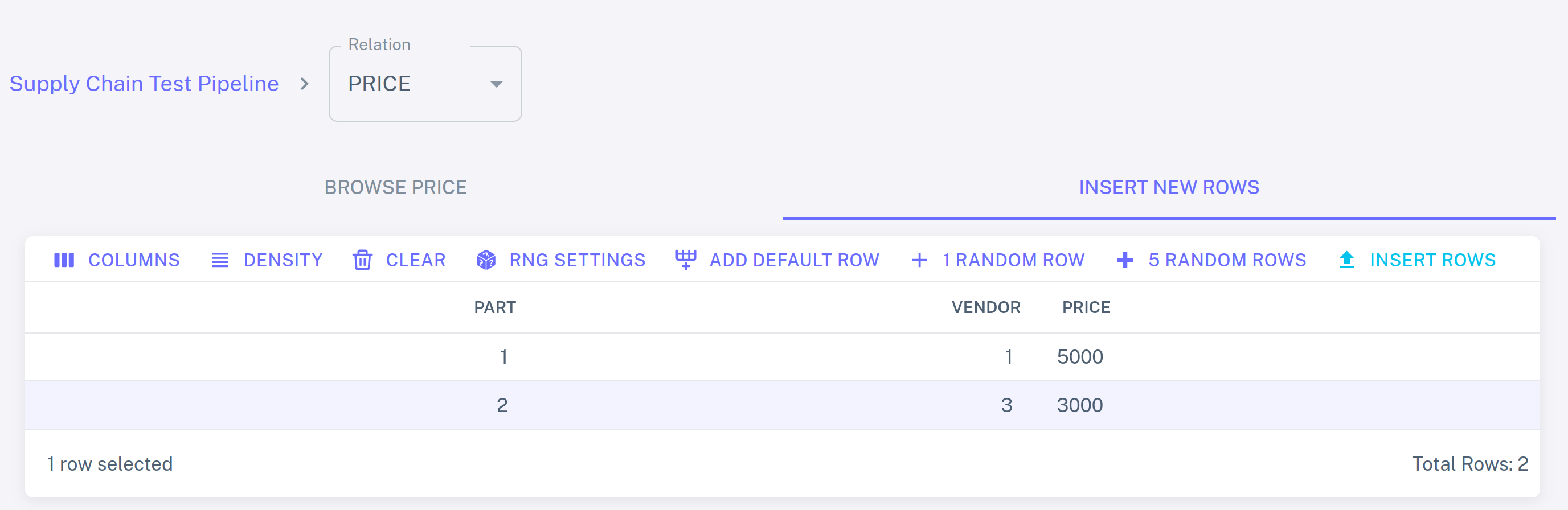
Click INSERT ROWS and switch back to the PREFERRED_VENDOR view. The view has changed: DarkMatter Devices is now the cheapest supplier of Warp Cores, while Gravitech Dynamics offers lowest-priced Flux Capacitors.

As you make more changes to the input tables, Feldera will keep updating the view.

This simple example illustrates the concept of continuous analytics. Feldera queries are always-on: the query engine continuously updates all views in response to input changes, making the most up-to-date results available at any time.

note

The Web Console does not yet support deleting records. Use the REST API described in the next part of the tutorial instead.

Step 6. Stop the pipeline

Click the stop icon to shut down the pipeline.

caution

All pipeline state will be lost.

Takeaways

Let us recap what we have learned so far:

• Feldera executes programs written in standard SQL, using CREATE TABLE and CREATE VIEW statements.

  • CREATE TABLE statements define a schema for input data.
  • CREATE VIEW statements define queries over input tables and other views.

• A SQL program is instantiated as part of a pipeline.

• Feldera evaluates queries continuously, updating their results as input data changes.